

The VLOOKUP function in Microsoft Excel is a powerful tool for finding information in a table based on a matching value. It is commonly used to retrieve product prices, employee details, customer information, inventory data, and other related records from large spreadsheets.
If you regularly work with Excel tables, learning how to use VLOOKUP can save time and reduce the need to search for information manually.
What Is the VLOOKUP Function in Excel?
VLOOKUP stands for Vertical Lookup. The function searches for a value in the first column of a selected table and returns related information from another column in the same row.
The basic syntax is:
=VLOOKUP(lookup_value, table_array, col_index_num, [range_lookup])
Each argument has a specific purpose:
- lookup_value – The value you want Excel to find.
- table_array – The range containing the data you want to search.
- col_index_num – The column number containing the result you want to return.
- range_lookup – Determines whether Excel should find an exact or approximate match.
How to Use VLOOKUP in Microsoft Excel
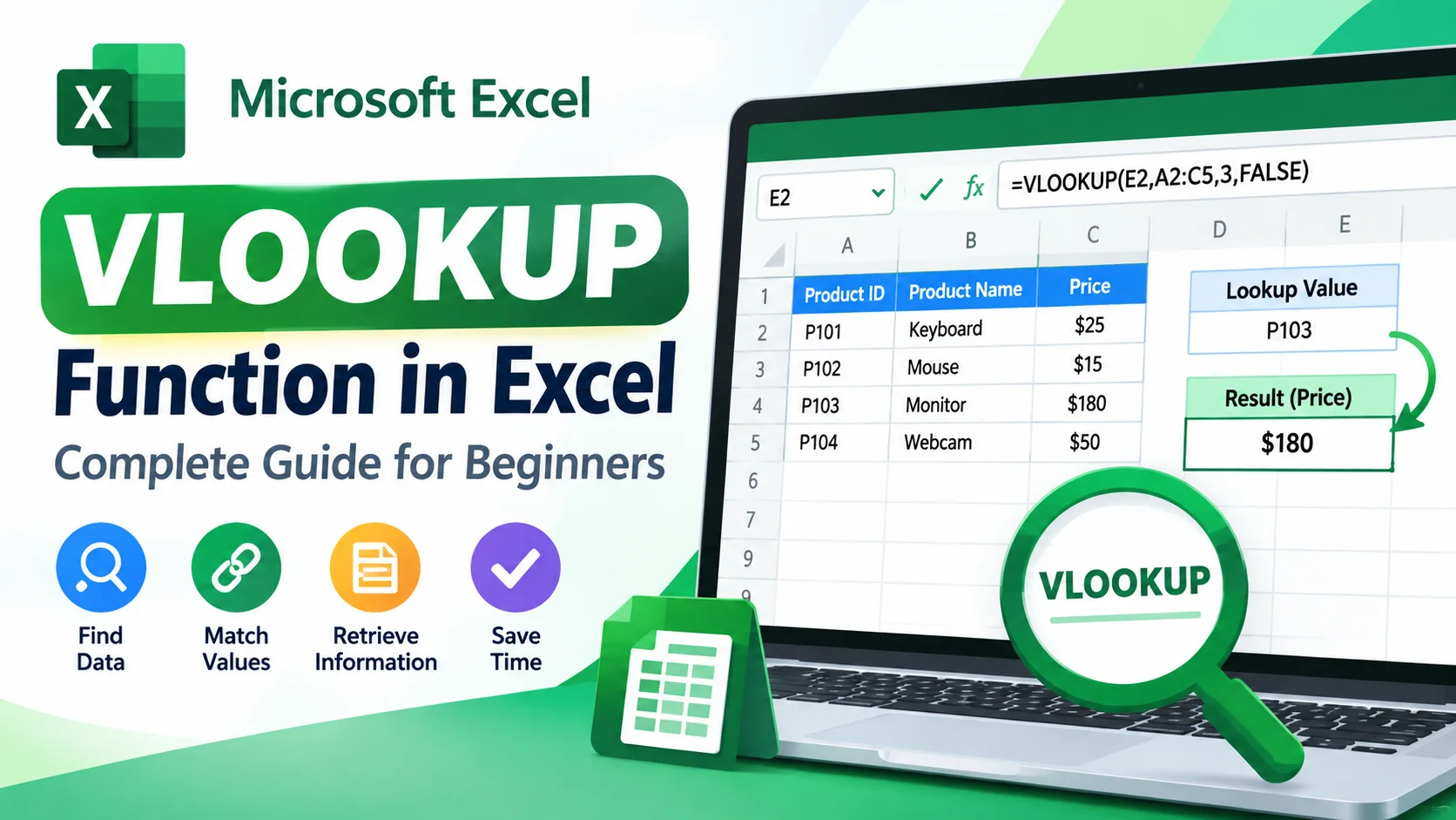
Suppose you have a product table like this:
| Product ID | Product Name | Price |
|---|---|---|
| P101 | Keyboard | $25 |
| P102 | Mouse | $15 |
| P103 | Monitor | $180 |
| P104 | Webcam | $50 |
If cell E2 contains P103 and you want to find the product price, you can use:
=VLOOKUP(E2,A2:C5,3,FALSE)
Excel searches for P103 in the first column of the table and returns the value from the third column.
The result is:
$180
Exact Match vs. Approximate Match
One of the most important parts of VLOOKUP is the final argument.
Exact Match
Use FALSE when you need an exact match:
=VLOOKUP(E2,A2:C5,3,FALSE)
This is usually the safest option for product IDs, employee IDs, invoice numbers, and other unique identifiers.
You can also use 0 instead of FALSE:
=VLOOKUP(E2,A2:C5,3,0)
Approximate Match
Use TRUE when you want an approximate match:
=VLOOKUP(E2,A2:C5,3,TRUE)
Approximate matching can be useful for ranges such as grades, tax brackets, discounts, or commission levels. The lookup column should be sorted appropriately for reliable results.
How to Use VLOOKUP Across Worksheets
VLOOKUP can retrieve information from another worksheet.
For example:
=VLOOKUP(A2,Products!A2:D100,4,FALSE)
This formula searches for the value in A2 within the Products worksheet and returns data from the fourth column.
This is useful when your workbook separates information into different sheets, such as:
- Products
- Customers
- Employees
- Orders
- Inventory
Using VLOOKUP With IFERROR
Sometimes VLOOKUP cannot find a matching value and returns the #N/A error.
You can make the result easier to understand by combining VLOOKUP with IFERROR:
=IFERROR(VLOOKUP(A2,Products!A2:C100,3,FALSE),"Not Found")
Instead of displaying #N/A, Excel displays:
Not Found
This is particularly useful when creating reports or user-friendly spreadsheets.
Common VLOOKUP Errors
#N/A
The lookup value could not be found.
Check whether:
- The lookup value exists.
- Spelling is correct.
- Extra spaces are present.
- The lookup column contains the correct data type.
#REF!
The column number is outside the selected table range.
For example:
=VLOOKUP(A2,A2:C20,5,FALSE)
The table only has three columns, so column 5 does not exist.
#VALUE!
This can occur when an argument contains an invalid value or when the formula structure is incorrect.
Incorrect Results
Incorrect results can occur when TRUE is used unintentionally or when an approximate lookup table is not properly sorted.
For most ID-based searches, use FALSE.
Important VLOOKUP Limitations
VLOOKUP is useful, but it has some limitations.
First, the lookup value must be located in the first column of the selected table.
For example, if the product name is in column B and the product ID is in column A, VLOOKUP can search for the product ID and return the product name. However, it cannot normally search column B and return a value from column A.
VLOOKUP also uses a column number rather than a column reference. If you insert or remove columns inside the lookup range, the formula may need to be updated.
VLOOKUP vs. XLOOKUP
Microsoft Excel also includes the newer XLOOKUP function, which provides more flexibility than VLOOKUP.
For example:
=XLOOKUP(E2,A2:A5,C2:C5,"Not Found")
XLOOKUP can search in different directions and does not require you to specify a numeric column index.
However, VLOOKUP remains important because it is widely used in existing Excel workbooks and is supported by many older Excel versions.
Tips for Using VLOOKUP Effectively
Follow these tips to avoid common problems:
- Use
FALSEfor most exact-match searches. - Make sure the lookup value is in the first column of the table.
- Check for extra spaces in text values.
- Use
IFERRORwhen you want cleaner results. - Use absolute references when copying formulas.
- Keep lookup tables organized and consistent.
- Use Excel Tables when working with frequently changing data.
For example:
=VLOOKUP(E2,$A$2:$C$100,3,FALSE)
The dollar signs prevent the lookup range from moving when the formula is copied to another cell.
Frequently Asked Questions
What is VLOOKUP used for in Excel?
VLOOKUP is used to search for a value in the first column of a table and return related information from another column in the same row.
What does FALSE mean in VLOOKUP?
FALSE tells Excel to look for an exact match. It is commonly recommended when searching for IDs, names, codes, or other specific values.
Can VLOOKUP search another sheet?
Yes. You can include another worksheet’s name in the table range, such as:
=VLOOKUP(A2,Sheet2!A:C,3,FALSE)
Why does VLOOKUP return #N/A?
The #N/A error usually means Excel cannot find the lookup value. Check the spelling, spaces, data type, and lookup range.
Is XLOOKUP better than VLOOKUP?
XLOOKUP offers additional flexibility and can overcome several VLOOKUP limitations. However, VLOOKUP remains useful for compatibility with existing workbooks and older Excel versions.
Conclusion
The VLOOKUP function in Microsoft Excel makes it easier to retrieve related information from tables without manually searching through rows. By understanding lookup values, table ranges, column indexes, and exact matching, you can use VLOOKUP effectively for spreadsheets involving products, customers, employees, inventory, and financial data.
For new Excel users, mastering VLOOKUP is an important step toward creating faster and more efficient spreadsheets. Once you understand VLOOKUP, you can also explore more advanced functions such as XLOOKUP, INDEX, and MATCH.