

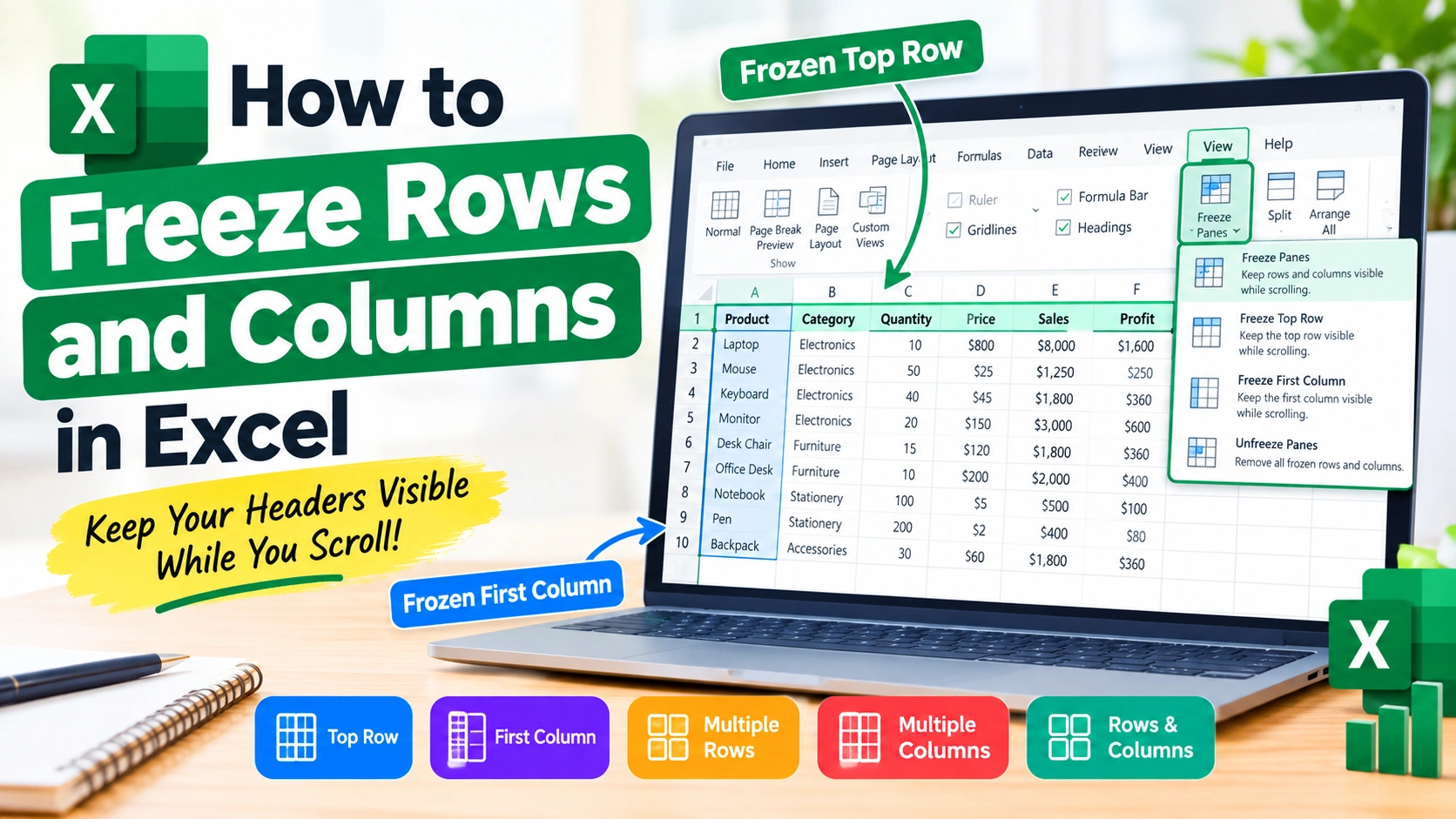
When working with a large spreadsheet, keeping track of your data can become difficult. As you scroll down hundreds of rows or move across dozens of columns, important headings can disappear from view. Fortunately, Microsoft Excel includes a useful feature called Freeze Panes that keeps selected rows or columns visible while you navigate through a worksheet.
Whether you’re managing a sales report, tracking inventory, analyzing financial data, or organizing a customer list, learning how to freeze rows and columns in Excel can make your spreadsheets much easier to use.
In this guide, you’ll learn how to freeze the top row, freeze the first column, freeze multiple rows or columns, freeze both rows and columns at the same time, and remove frozen panes when you no longer need them.
What Does Freeze Panes Do in Excel?
The Freeze Panes feature locks specific rows or columns in place so they remain visible while you scroll through the rest of the worksheet.
For example, imagine a spreadsheet with these column headings:
- Product
- Category
- Quantity
- Price
- Sales
- Profit
If the spreadsheet contains hundreds of records, the headings may disappear when you scroll down. By freezing the top row, the column headings remain visible, making it easier to understand the information you’re viewing.
Freezing panes does not change the position of your data permanently. It simply keeps selected rows or columns visible while you scroll.
How to Freeze the Top Row in Excel
Freezing the top row is one of the easiest ways to keep column headings visible.
Step 1: Open Your Excel Worksheet
Open the workbook containing the spreadsheet you want to work with.
Step 2: Go to the View Tab
At the top of Excel, select the View tab.
Step 3: Open Freeze Panes
Look for the Freeze Panes option in the Window section of the ribbon.
Click it to display the available options.
Step 4: Select Freeze Top Row
Choose Freeze Top Row.
Excel will immediately lock the first row in place.
Now, when you scroll downward, the first row will remain visible at the top of the worksheet.
How to Freeze the First Column in Excel
If your spreadsheet contains important information in the first column, you can keep it visible while scrolling horizontally.
To freeze the first column:
- Open your Excel worksheet.
- Select the View tab.
- Click Freeze Panes.
- Select Freeze First Column.
The first column will remain visible as you scroll from left to right.
This is particularly useful when the first column contains names, product IDs, account numbers, or other information that helps identify each row.
How to Freeze Multiple Rows in Excel
Excel also lets you freeze several rows instead of just the top row.
Suppose your spreadsheet has three rows containing titles, headings, and additional information that you want to keep visible.
Follow these steps:
- Click the row directly below the rows you want to freeze.
- Select the View tab.
- Click Freeze Panes.
- Choose Freeze Panes from the menu.
For example, if you want to freeze rows 1 through 3, select a cell in row 4 before choosing Freeze Panes.
Excel will freeze everything above the selected cell.
Important Rule for Freezing Rows
The key is to select the row below the rows you want to keep visible.
For example:
| Rows You Want to Freeze | Select |
|---|---|
| Row 1 | Row 2 |
| Rows 1–2 | Row 3 |
| Rows 1–3 | Row 4 |
| Rows 1–5 | Row 6 |
This same principle applies when freezing columns.
How to Freeze Multiple Columns in Excel
You can also freeze more than one column.
For example, suppose columns A and B contain customer names and customer IDs, and you want them to remain visible while scrolling horizontally.
Follow these steps:
- Select the column immediately to the right of the columns you want to freeze.
- Go to View.
- Click Freeze Panes.
- Select Freeze Panes.
To freeze columns A and B, select a cell in column C before activating Freeze Panes.
Excel will keep columns A and B visible while you scroll horizontally.
How to Freeze Rows and Columns at the Same Time
One of the most useful Excel features is the ability to freeze both rows and columns simultaneously.
This is especially helpful for large tables where you need to keep column headings and identifying information visible.
For example, suppose:
- Row 1 contains your column headings.
- Column A contains product names.
You can freeze both at the same time.
Follow These Steps
- Click the cell immediately below the row and immediately to the right of the column you want to freeze.
- Open the View tab.
- Click Freeze Panes.
- Select Freeze Panes again.
For example, if you want to freeze the first row and first column, select cell B2.
Excel will keep:
- Row 1 visible when scrolling vertically.
- Column A visible when scrolling horizontally.
This is particularly useful for large datasets because you can always see both the column headings and the information identifying each row.
How to Freeze the Top Two Rows and First Column
You aren’t limited to freezing just one row or column.
Suppose you want to freeze:
- Rows 1 and 2
- Column A
Select cell B3.
Then:
- Go to View.
- Click Freeze Panes.
- Select Freeze Panes.
Everything above and to the left of the selected cell will remain visible.
This method gives you precise control over which rows and columns stay on screen.
How to Unfreeze Rows and Columns in Excel
If you no longer need frozen panes, you can easily remove them.
Step 1: Open the View Tab
Click View in the Excel ribbon.
Step 2: Select Freeze Panes
Click Freeze Panes.
Step 3: Choose Unfreeze Panes
Select Unfreeze Panes.
The worksheet will return to normal scrolling.
Your data will not be deleted or rearranged. Unfreezing simply removes the locked scrolling areas.
Freeze Panes vs. Split Panes
Excel includes another feature called Split that can sometimes be confused with Freeze Panes.
Although both affect how you view a worksheet, they work differently.
Freeze Panes keeps selected rows or columns visible while you scroll.
Split divides the worksheet window into separate viewing areas. Each area can be scrolled independently.
For most situations where you simply want headings or labels to remain visible, Freeze Panes is the more straightforward option.
Common Problems When Freezing Rows and Columns
Sometimes Freeze Panes may not work as expected. Here are some common issues and solutions.
You Froze the Wrong Rows
If the wrong rows remain visible, you probably selected the wrong cell before choosing Freeze Panes.
Remember that Excel freezes the rows above and columns to the left of the selected cell.
Unfreeze the panes and select the correct cell before trying again.
Freeze Panes Is Grayed Out
Certain worksheet situations or modes can affect the availability of some Excel commands.
If Freeze Panes is unavailable, check whether you’re currently editing a cell, using a special worksheet view, or working with a protected worksheet.
Press Esc or Enter to exit cell-editing mode and try again.
You Want to Freeze a Row That Isn’t at the Top
Excel’s Freeze Panes feature is designed around the rows above your selected cell. You cannot simply choose an arbitrary middle row and freeze only that row while allowing the rows above it to scroll normally.
If you need a different viewing arrangement, consider using Split or reorganizing the worksheet.
Tips for Using Freeze Panes Effectively
Freeze Panes is most useful when applied strategically. Consider these tips when working with large Excel spreadsheets.
Keep Header Rows Visible
If your worksheet has a single row of column headings, freezing the top row is usually enough.
Freeze Identifier Columns
If the first column contains customer names, employee names, product codes, or other identifiers, freezing it can make large tables easier to navigate.
Avoid Freezing Too Much
Freezing several rows and columns can reduce the amount of space available for your data.
Only freeze information that you genuinely need to reference while scrolling.
Check Your Worksheet Before Sharing
If you’re sending an Excel workbook to someone else, check the frozen panes first. A view that works well for you may not be ideal for another person.
When Should You Use Freeze Panes?
Freeze Panes is particularly useful when working with:
- Large sales reports
- Inventory spreadsheets
- Employee lists
- Financial reports
- Customer databases
- Project trackers
- Attendance records
- Budget worksheets
- Data analysis tables
- Monthly or yearly reports
If you frequently scroll through a spreadsheet and lose track of what each row or column represents, Freeze Panes can make the worksheet significantly easier to navigate.
Frequently Asked Questions
Can I freeze more than one row in Excel?
Yes. Select the row immediately below the rows you want to freeze, then choose View > Freeze Panes > Freeze Panes.
Can I freeze more than one column?
Yes. Select the column immediately to the right of the columns you want to freeze, then activate Freeze Panes.
Can I freeze rows and columns together?
Yes. Select the cell below and to the right of the rows and columns you want to freeze, then choose Freeze Panes.
Does freezing panes change my spreadsheet data?
No. Freeze Panes only changes how the worksheet behaves while scrolling. It does not modify, delete, or rearrange your data.
How do I remove frozen panes?
Go to View > Freeze Panes > Unfreeze Panes.
Why can’t I freeze a specific middle row by itself?
Freeze Panes locks the rows above the selected cell. It does not allow you to freeze an isolated middle row while the rows above it continue scrolling normally.
Final Thoughts
Learning how to freeze rows and columns in Excel is a simple skill that can make a major difference when working with large spreadsheets. By keeping headings, labels, and important identifiers visible, you can navigate extensive worksheets without constantly scrolling back to the top or left side.
For a basic worksheet, Freeze Top Row or Freeze First Column may be all you need. For larger spreadsheets, you can select a specific cell and use Freeze Panes to lock multiple rows and columns at the same time.
Once you get familiar with how Excel determines which areas to freeze, you can quickly customize the worksheet view to make your data easier to read and manage.